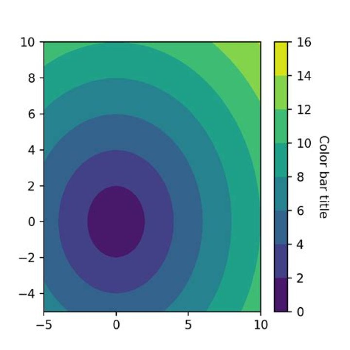
I can't seem to find the answer anywhere! I found a discussion here, but trying this I get a TypeError: 'NoneType' object is not iterable:
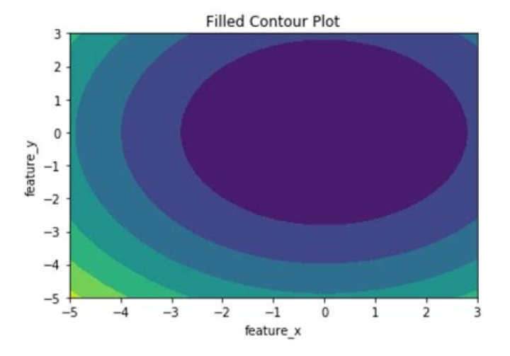
>>> import numpy as np >>> import matplotlib.pyplot as plt >>> x, y = np.meshgrid(np.arange(10),np.arange(10)) >>> z = x + y >>> cs = plt.contourf(x,y,z,levels=[2,3]) >>> cs.collections[0].set_label('test') >>> plt.legend() Traceback (most recent call last): File "<stdin>", line 1, in <module> File "/opt/local/Library/Frameworks/", line 2791, in legend ret = gca().legend(*args, **kwargs) File "/opt/local/Library/Frameworks/", line 4475, in legend self.legend_ = mlegend.Legend(self, handles, labels, **kwargs) File "/opt/local/Library/Frameworks/", line 365, in __init__ self._init_legend_box(handles, labels) File "/opt/local/Library/Frameworks/", line 627, in _init_legend_box handlebox) File "/opt/local/Library/Frameworks/", line 110, in __call__ handlebox.get_transform()) File "/opt/local/Library/Frameworks/", line 352, in create_artists width, height, fontsize) File "/opt/local/Library/Frameworks/", line 307, in get_sizes size_max = max(orig_handle.get_sizes())*legend.markerscale**2 TypeError: 'NoneType' object is not iterable EDIT: I'm looking for something like this:
4 Answers
You could also do it directly with the lines of the contour, without using proxy artists.
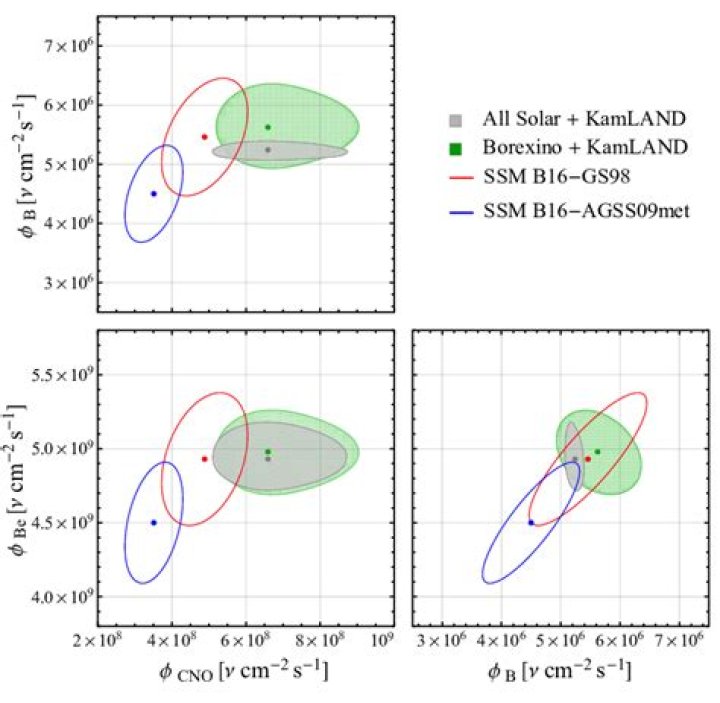
import matplotlib import numpy as np import matplotlib.cm as cm import matplotlib.mlab as mlab import matplotlib.pyplot as plt matplotlib.rcParams['xtick.direction'] = 'out' matplotlib.rcParams['ytick.direction'] = 'out' delta = 0.025 x = np.arange(-3.0, 3.0, delta) y = np.arange(-2.0, 2.0, delta) X, Y = np.meshgrid(x, y) Z1 = mlab.bivariate_normal(X, Y, 1.0, 1.0, 0.0, 0.0) Z2 = mlab.bivariate_normal(X, Y, 1.5, 0.5, 1, 1) # difference of Gaussians Z = 10.0 * (Z2 - Z1) # Create a simple contour plot with labels using default colors. The # inline argument to clabel will control whether the labels are draw # over the line segments of the contour, removing the lines beneath # the label plt.figure() CS = plt.contour(X, Y, Z) plt.clabel(CS, inline=1, fontsize=10) plt.title('Simplest default with labels') labels = ['line1', 'line2','line3','line4', 'line5', 'line6'] for i in range(len(labels)): CS.collections[i].set_label(labels[i]) plt.legend(loc='upper left') Will produce:

However, you might also want to look into annotations for your own need. In my opinion it will give you a more fine grained control on where and what you write on the image, here is the same example with some annotation:
### better with annotation, more flexible plt.figure(2) CS = plt.contour(X, Y, Z) plt.clabel(CS, inline=1, fontsize=10) plt.title('Simplest default with labels') plt.annotate('some text here',(1.4,1.6)) plt.annotate('some text there',(-2,-1.5)) 
You can create proxy artists to make the legend:
import numpy as np import matplotlib.pyplot as plt x, y = np.meshgrid(np.arange(10),np.arange(10)) z = np.sqrt(x**2 + y**2) cs = plt.contourf(x,y,z,levels=[2,3,4,6]) proxy = [plt.Rectangle((0,0),1,1,fc = pc.get_facecolor()[0]) for pc in cs.collections] plt.legend(proxy, ["range(2-3)", "range(3-4)", "range(4-6)"]) plt.show() 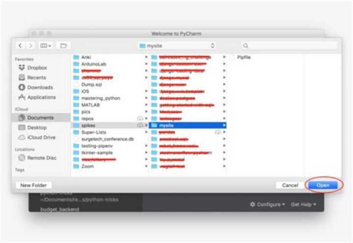
I had a similar question but needed to go a bit beyond HYRY's answer. To make a package user friendly I wanted ax.legend() to work without requiring users to pass any handles, which can be achieved by passing the label on to the proxy
proxy = plt.Rectangle((0, 0), 1, 1, fc='red', label='some label') and then adding the proxy to the axis' patches:
ax.patches += [proxy] (do ax = plt.gca() to get the current axis)
This is described in more detail in this answer.
Adding to this answer to make it less manual:
import numpy as np import matplotlib.pyplot as plt x, y = np.meshgrid(np.arange(10),np.arange(10)) z = np.sqrt(x**2 + y**2) levels=[2,3,4,6] cs = plt.contourf(x,y,z,levels=levels) proxy = [plt.Rectangle((0,0),1,1,fc = pc.get_facecolor()[0]) for pc in cs.collections] plt.legend(proxy, [f"{lower:2.1f} - {upper:2.1f}" for lower, upper in zip(levels[:-1], levels[1:])]) plt.show()