I'm trying to create a simple spreadsheet that contains tables for a Budget (By Category) and a list of Transactions (With each transaction belonging to a Category), and then a Pivot Table showing a summary of the Budget and Actual Spending by Category.
The basics are working fine, as shown below:
 (The Blue table is Transactions, Green is Budget and the Pink table is the Pivot table)
To get the Pivot Table to work as shown above I had to create a Relationship, as shown below:
All good so far. The problem is that I now want to add another column to the Pivot table showing the remaining budget/overspend. i.e. The Budget for a category minus the amount spent for that category so far. (Or =Column2 - Column3)
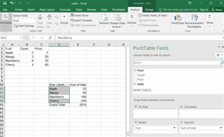
Everything I've read online says I need to add a "Calculated Field" from under the "Fields, Items & Sets" menu, however this is Greyed Out for me:
I searched for why this would be greyed out and all I can find is that "Calculated Fields" cannot be added for OLAP sourced data, but my data is not OLAP sourced.
Help would be appreciated.
Thanks Ben
11 Answer
It doesn't work since you have a relationship (i.e. you have added the tables to a data model).
In my experience the calculated field is very beneficially when you work with a single table without much complexity.
In the following scenarios the "calculated field" will be disabled
- If the pivot table is based on OLAP source data
- If you have external data sources
- If you click "Add this data to the Data Model" when you create PivotTable
To achieve what you want you would need to use a "Measure".
Enter the following formula, which I call "Left to spend". (Sum of Budget can you get if you drag the Budget field "values" in the PivotTable, as you already have done in your print screen):
=SUMX(Budget,[Sum of Budget]-[Sum of Amount])
You could then arrange your pivot table like this: