I have a set of coordinates:
d1 <- data_frame( title = c("base1", "base2", "base3", "base4"), lat = c(57.3, 58.8, 47.2, 57.8, 65.4, 56.7, 53.3), long = c(0.4, 3.4, 3.5, 1.2, 1.5, 2.6, 2.7)) I would like to know whether the coordinates fall on land, in the sea, or are 3 miles inside a coastline. The coordinates should fall somewhere within the UK, so I know that I need to draw a shape file of the UK and plot the points onto it.
I just don't know how to measure whether the points fall in the sea, land or 2 miles from the coast. Obviously I can tell from looking at a map where they fall, but what I would like is to add another column to my data set so it looks like this:
d2 <- data_frame( title = c("base1", "base2", "base3", "base4", "base5", "base6", "base7"), lat = c(57.3, 58.8, 47.2, 57.8, 65.4, 56.7, 53.3), long = c(0.4, 3.4, 3.5, 1.2, 1.5, 2.6, 2.7), where = c("land", "land", "sea", "coast", "land", "sea", "coast")) - note that the data in d2 column 'where' is illustrative, these lat/long points may all be on land, or something else
4 Answers
Distance to the coastline can be calculated by downloading openstreetmap coastline data. You can then use geosphere::dist2Line to get the distance from your points to the coastline.
I noticed that one of your example points was in France so you may need to expand the coastline data beyond just the UK (can be done by playing with the extents of the bounding box).
library(tidyverse) library(sf) library(geosphere) library(osmdata) #get initial data frame d1 <- data_frame( title = c("base1", "base2", "base3", "base4", "base5", "base6", "base7"), lat = c(57.3, 58.8, 47.2, 57.8, 65.4, 56.7, 53.3), long = c(0.4, 3.4, 3.5, 1.2, 1.5, 2.6, 2.7)) # convert to sf object d1_sf <- d1 %>% st_as_sf(coords = c('long','lat')) %>% st_set_crs(4326) # get bouding box for osm data download (England) and # download coastline data for this area osm_box <- getbb (place_name = "England") %>% opq () %>% add_osm_feature("natural", "coastline") %>% osmdata_sf() # use dist2Line from geosphere - only works for WGS84 #data dist <- geosphere::dist2Line(p = st_coordinates(d1_sf), line = st_coordinates(osm_box$osm_lines)[,1:2]) #combine initial data with distance to coastline df <- cbind( d1 %>% rename(y=lat,x=long),dist) %>% mutate(miles=distance/1609) # title y x distance lon lat miles #1 base1 57.3 0.4 219066.40 -2.137847 55.91706 136.15065 #2 base2 58.8 3.4 462510.28 -2.137847 55.91706 287.45201 #3 base3 47.2 3.5 351622.34 1.193198 49.96737 218.53470 #4 base4 57.8 1.2 292210.46 -2.137847 55.91706 181.60998 #5 base5 65.4 1.5 1074644.00 -2.143168 55.91830 667.89559 #6 base6 56.7 2.6 287951.93 -1.621963 55.63143 178.96329 #7 base7 53.3 2.7 92480.24 1.651836 52.76027 57.47684 #plot p <- ggplot() + geom_sf(data=osm_box$osm_lines) + geom_sf(data=d1_sf) + geom_segment(data=df,aes(x=x,y=y,xend=lon,yend=lat)) 
That's just for the distance to the coastline. You also need to know how whether it is inland or at sea. For this, you would need a separate shapefile for the sea: and see if each point of your points sits in the sea or not.
#read in osm water polygon data sea <- read_sf('water_polygons.shp') #get get water polygons that intersect our points in_sea <- st_intersects(d1_sf,sea) %>% as.data.frame() #join back onto original dataset df %>% mutate(row = row_number()) %>% #join on in_sea data left_join(in_sea,by=c('row'='row.id')) %>% mutate(in_sea = if_else(is.na(col.id),F,T)) %>% #categorise into 'sea', 'coast' or 'land' mutate(where = case_when(in_sea == T ~ 'Sea', in_sea == F & miles <=3 ~ 'Coast', in_sea == F ~ 'Land')) # title y x distance lon lat miles row col.id in_sea where #1 base1 57.3 0.4 219066.40 -2.137847 55.91706 136.15065 1 24193 TRUE Sea #2 base2 58.8 3.4 462510.28 -2.137847 55.91706 287.45201 2 24194 TRUE Sea #3 base3 47.2 3.5 351622.34 1.193198 49.96737 218.53470 3 NA FALSE Land #4 base4 57.8 1.2 292210.46 -2.137847 55.91706 181.60998 4 24193 TRUE Sea #5 base5 65.4 1.5 1074644.00 -2.143168 55.91830 667.89559 5 25417 TRUE Sea #6 base6 56.7 2.6 287951.93 -1.621963 55.63143 178.96329 6 24193 TRUE Sea #7 base7 53.3 2.7 92480.24 1.651836 52.76027 57.47684 7 24143 TRUE Sea ggplot() + geom_sf(data=osm_box$osm_lines) + geom_sf(data=d1_sf) + geom_segment(data=df,aes(x=x,y=y,xend=lon,yend=lat)) + ggrepel::geom_text_repel(data=df, aes(x=x,y=y,label=paste0(where,'\n',round(miles,0),'miles')),size=2)
Update 16/08/2018
Since you asked for an approach specifically using a shapefile I have downloaded this one here: which I will use to carry out the same approach as above.
clines <- read_sf('lines.shp') #path to shapefile Next I created a custom bounding box so that we can cut down the size of the shapefile to only include coastlines reasonably close to the points.
# create bounding box surrounding points bbox <- st_bbox(d1_sf) # write a function that takes the bbox around our points # and expands it by a given amount of metres. expand_bbox <- function(bbox,metres_x,metres_y){ box_centre <- bbox %>% st_as_sfc() %>% st_transform(crs = 32630) %>% st_centroid() %>% st_transform(crs = 4326) %>% st_coordinates() bbox['xmin'] <- bbox['xmin'] - (metres_x / 6370000) * (180 / pi) / cos(bbox['xmin'] * pi/180) bbox['xmax'] <- bbox['xmax'] + (metres_x / 6370000) * (180 / pi) / cos(bbox['xmax'] * pi/180) bbox['ymin'] <- bbox['ymin'] - (metres_y / 6370000) * (180 / pi) bbox['ymax'] <- bbox['ymax'] + (metres_y / 6370000) * (180 / pi) bbox['xmin'] <- ifelse(bbox['xmin'] < -180, bbox['xmin'] + 360, bbox['xmin']) bbox['xmax'] <- ifelse(bbox['xmax'] > 180, bbox['xmax'] - 360, bbox['xmax']) bbox['ymin'] <- ifelse(bbox['ymin'] < -90, (bbox['ymin'] + 180)*-1, bbox['ymin']) bbox['ymax'] <- ifelse(bbox['ymax'] > 90, (bbox['ymax'] + 180)*-1, bbox['ymax']) return(bbox) } # expand the bounding box around our points by 300 miles in x and 100 #miles in y direction to make nice shaped box. bbox <- expand_bbox(bbox,metres_x=1609*200, metres_y=1609*200) %>% st_as_sfc # get only the parts of the coastline that are within our bounding box clines2 <- st_intersection(clines,bbox) Now I used the dist2Line function here because it is accurate and it gives you the points on the coastline it is measuring to which makes it good for checking errors. The downside is, it's very slow for our rather large coastline file.
Running this took me 8 minutes:
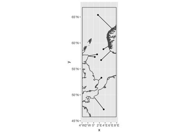
dist <- geosphere::dist2Line(p = st_coordinates(d1_sf), line = as(clines2,'Spatial')) #combine initial data with distance to coastline df <- cbind( d1 %>% rename(y=lat,x=long),dist) %>% mutate(miles=distance/1609) df # title y x distance lon lat ID miles #1 base1 57.3 0.4 131936.70 -1.7711149 57.46995 4585 81.99919 #2 base2 58.8 3.4 98886.42 4.8461433 59.28235 179 61.45831 #3 base3 47.2 3.5 340563.02 0.3641618 49.43811 4199 211.66129 #4 base4 57.8 1.2 180110.10 -1.7670712 57.50691 4584 111.93915 #5 base5 65.4 1.5 369550.43 6.2494627 62.81381 9424 229.67709 #6 base6 56.7 2.6 274230.37 5.8635346 58.42913 24152 170.43528 #7 base7 53.3 2.7 92480.24 1.6518358 52.76027 4639 57.47684 plot:
ggplot() + geom_sf(data=clines2) + geom_sf(data=bbox,fill=NA)+ geom_sf(data=d1_sf) + geom_segment(data=df,aes(x=x,y=y,xend=lon,yend=lat))
If you don't mind about the slight loss of accuracy (results differ by around 0.3% on your data), and are not fussed about knowing where exactly on the coastline it is measuring to, you can measure the distance to the polygon:
# make data into polygons clines3 <- st_intersection(clines,bbox) %>% st_cast('POLYGON') #use rgeos::gDistance to calculate distance to nearest polygon #need to change projection (I used UTM30N) to use gDistance dist2 <- apply(rgeos::gDistance(as(st_transform(d1_sf,32630), 'Spatial'), as(st_transform(clines3,32630),'Spatial'), byid=TRUE),2,min) df2 <- cbind( d1 %>% rename(y=lat,x=long),dist2) %>% mutate(miles=dist2/1609) df2 # title y x dist2 miles #1 base1 57.3 0.4 131917.62 81.98733 #2 base2 58.8 3.4 99049.22 61.55949 #3 base3 47.2 3.5 341015.26 211.94236 #4 base4 57.8 1.2 180101.47 111.93379 #5 base5 65.4 1.5 369950.32 229.92562 #6 base6 56.7 2.6 274750.17 170.75834 #7 base7 53.3 2.7 92580.16 57.53894 By contrast this took just 8 seconds to run!
The rest is as in the previous answer.
7There is a simple way to do this using the ggOceanMaps package
library(ggOceanMaps) library(dplyr) d1 <- data.frame( title = c("base1", "base2", "base3", "base4", "base5", "base6", "base7"), lat = c(57.3, 58.8, 47.2, 57.8, 65.4, 56.7, 53.3), long = c(0.4, 3.4, 3.5, 1.2, 1.5, 2.6, 2.7)) ggOceanMaps::dist2land(d1) %>% mutate(where = ifelse(ldist == 0, "land", ifelse(ldist < 100*1.852, "coast", "sea"))) #> Used long and lat as input coordinate column names in data #> Using ArcticStereographic as land shapes. #> Calculating distances with parallel processing... #> title lat long ldist where #> 1 base1 57.3 0.4 138.62996 coast #> 2 base2 58.8 3.4 105.43322 coast #> 3 base3 47.2 3.5 0.00000 land #> 4 base4 57.8 1.2 189.78665 sea #> 5 base5 65.4 1.5 382.64410 sea #> 6 base6 56.7 2.6 289.76883 sea #> 7 base7 53.3 2.7 99.18336 coast The ggOceanMaps::dist2land function returns distances in kilometers. I converted to nautical miles and pumped up the limit to get all different categories. Your example coordinates would have yielded one case of "land" and the rest as "sea".
Created on 2021-12-01 by the reprex package (v2.0.1)
First you need a file containing coastlines of UK.
You can use the method provided in this question to know whether a point falls inside the UK coastlines or outside.
Then, for points that fall into the UK, you can compute the Haversine distance between them and the coast line points, to determine if they are in your 3 miles from the coast.
For a faster implementation of geosphere:::dist2Line that uses purrr for efficient looping and progress for a progress bar, thus retaining the accuracy of Chris' first answer, see below:
library(geosphere) library(purr) library(progress) spDistPoint2Line <- function (p, line, distfun) { ## rewrite of internal function from geosphere test <- !sp::is.projected(line) if (!isTRUE(test)) { if (is.na(test)) { warning("Coordinate reference system of SpatialPolygons object is not set. Assuming it is degrees (longitude/latitude)!") } else { stop("Points are projected. They should be in degrees (longitude/latitude)") } } x <- line@lines n <- length(x) res <- matrix(nrow = nrow(p), ncol = 3) colnames(res) <- c("distance", "lon", "lat") line_coords <- map(x, ~(map(.@Lines, ~(.@coords)))) #basically an unlist pb <- progress_bar$new( total = length(line_coords), format = "(:spin) :current of :total, :percent, eta: :eta" ) res[] <- Inf result <- reduce( .x = line_coords, .init = res, .f = function(res, crd){ pb$tick() crd <- crd[[1]] r <- dist2Line(p, crd, distfun) # have to live without ID k <- r[, 1] < res[, 1] res[k, ] <- r[k, ] return(res) } ) return(result) } dist2Line <- function (p, line, distfun = distGeo) { p <- geosphere:::.pointsToMatrix(p) if (inherits(line, "SpatialPolygons")) { line <- methods::as(line, "SpatialLines") } if (inherits(line, "SpatialLines")) { return(spDistPoint2Line(p, line, distfun)) } line <- geosphere:::.pointsToMatrix(line) line1 <- line[-nrow(line), , drop = FALSE] line2 <- line[-1, , drop = FALSE] seglength <- distfun(line1, line2) res <- p %>% array_branch(1) %>% map( function(xy){ crossdist <- abs(dist2gc(line1, line2, xy)) trackdist1 <- alongTrackDistance(line1, line2, xy) trackdist2 <- alongTrackDistance(line2, line1, xy) mintrackdist <- pmin(trackdist1, trackdist2) maxtrackdist <- pmax(trackdist1, trackdist2) crossdist[maxtrackdist >= seglength] <- NA nodedist <- distfun(xy, line) warnopt = getOption("warn") options(warn = -1) distmin1 <- min(nodedist, na.rm = TRUE) distmin2 <- min(crossdist, na.rm = TRUE) options(warn = warnopt) if (distmin1 <= distmin2) { j <- which.min(nodedist) return(c(distmin1, line[j, ])) } else { j <- which.min(crossdist) if (trackdist1[j] < trackdist2[j]) { bear <- bearing(line1[j, ], line2[j, ]) pt <- destPoint(line1[j, ], bear, mintrackdist[j]) return(c(crossdist[j], pt)) } else { bear <- bearing(line2[j, ], line1[j, ]) pt <- destPoint(line2[j, ], bear, mintrackdist[j]) return(c(crossdist[j], pt)) } } } ) %>% simplify %>% matrix(ncol = 3, byrow = TRUE) colnames(res) <- c("distance", "lon", "lat") return(res) }