How to get multi-row sort/filtering headers in excel

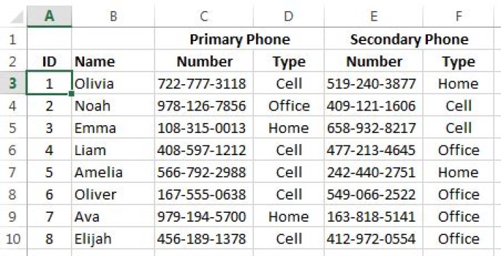
I have a spreadsheet which uses 2 rows for header information. Filtering by selecting a column is implicitly assuming only 1 row of header information. Sorting has a header row checkbox but that only toggles treating the first row as a header.

Is there a way to make Excel treat the first two rows as headers?

14 Answers

No. Omit the first row from your range when you auto filter. This way the auto filter buttons appear only on your bottom header row and the data gets filtered. I expect that right now your second header row is getting pulled into your 'data'.

You can't select a single cell and have excel figure this out. You have to select the range of cells you want excel to include.

An easy way to accomplish the sort function using multiple header rows is to insert a blank row just above the row you want to sort by (ideally, it is bottom-most in your header. If not, make it so.). Then click on the 'row' number highlighting the empty row. Right click that row and select "Hide'. The new, empty row will vanish leaving your header the way you wanted it to look and Excel will interpret your category row as the header.

If you select an entire row (by selecting the row number to the left of the row) and then enable your filter (Data > Filter) then it will give you filters for everything below the selected row and ignore everything above it.

To filter a list with 2 header rows, where the second row contains the column headings, here is what I did.

• Cut the first row
• Turn filtering off
• Turn filtering on again so that the second row is filtered. This tells Excel which is the row with the column headings.
• Paste the first row back in again above the row with the filters and column headings
• Check to see if the filter now works, with the column headings on the second row.

Okay, the following works in Excel 2010, even after saving the file back as an Excel 2007 and re-opening (so presumably works in Excel 2007 as well...)

Assuming a 3 row header. Set the spreadsheet filter range to Start at cell $A$4 and ensure that it covers the full extent of data you want to sort. SAVE THE FILE.

Henceforth, any sort will treat rows 1 to 3 as headers and therefore sort from row 4 onwards only. - UNLESS you change or cancel the filter range....

I know that I'm on SuperUser and not on StackOverflow, but the solution to this problem can be found in using VBA code on Excel 2016.

I have similar (more complex) problem.

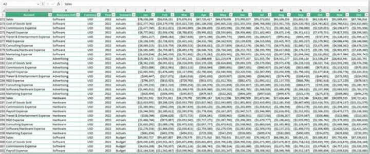
I want to add some filters on explicit columns but not on row 1 only on row 2 as you can see in following screen's capture.

I have tried using Excel GUI but this seems impossible, so I have written following code:

'******************************************************** '* SetFilter() '******************************************************** '* PUBLIC method to call to define CUSTOM AutoFilter '* on complex header. '******************************************************** Sub SetFilter() 'Compute last row number Dim nLast As Long nLast = Range("A" & Rows.Count).End(xlUp).Row 'Lock screen update Application.ScreenUpdating = False 'Unmerge merged cells to allow adding filter Range("A1:A2").MergeCells = False Range("B1:B2").MergeCells = False Range("C1:C2").MergeCells = False Range("D1:D2").MergeCells = False Range("E1:E2").MergeCells = False Range("F1:F2").MergeCells = False 'Add filter on row 2 and not 1 Range("A2:Z" & nLast).Select Selection.AutoFilter 'Remove (or Hide) filter combobox for some columns Selection.AutoFilter Field:=GetColumnIndex("C"), VisibleDropDown:=False Selection.AutoFilter Field:=GetColumnIndex("G"), VisibleDropDown:=False Selection.AutoFilter Field:=GetColumnIndex("H"), VisibleDropDown:=False 'Merge unmerged cells to restore previous state Range("A1:A2").MergeCells = True Range("B1:B2").MergeCells = True Range("C1:C2").MergeCells = True Range("D1:D2").MergeCells = True Range("E1:E2").MergeCells = True Range("F1:F2").MergeCells = True 'Unlock screen update Application.ScreenUpdating = True End Sub '******************************************************** '* GetColumnIndex() '******************************************************** '* return column's index from column letters '******************************************************** Function GetColumnIndex(sColLetter As String) As Integer Dim n As Integer: n = 0 Dim iMax As Integer: iMax = Len(sColLetter) Dim i As Integer Dim sChar As String Dim c As Integer For i = 1 To iMax sChar = Mid(sColLetter, i, 1) c = 1 + Asc(sChar) - Asc("A") n = n * 26 + c Next If n = 1 Then n = 1 End If GetColumnIndex = n End Function 

The logic of this code is

A. Unmerge vertically merged header cells to allow adding filter on row 2

Range("A1:A2").MergeCells = False 

Cells A1 and A2 are unmerged.

B. Add AutoFilter on all cells of row 2

Range("A2:Z" & nLast).AutoFilter 

AutoFilter is generated for cells in all rows except row 1.

C. Remove or hide FILTER Combobox for some columns

Selection.AutoFilter Field:=GetColumnIndex("C"), VisibleDropDown:=False 

DropBox of Column "C" is hidden.

D. Merge unmerged cells to restore original state

Range("A1:A2").MergeCells = True 

Cells A1 and A2 are merged again.

Is there a way to make Excel treat the first two rows as headers?

Yes there is, if you can make one small change to the first header column.

If you are able to merge cells A1 and A2 using "Merge & Center", then Excel will properly identify both rows as header rows.

For example:

Doing an auto-sort on this will automatically (and improperly) select the second row:

But now merge A1 and A2 together:

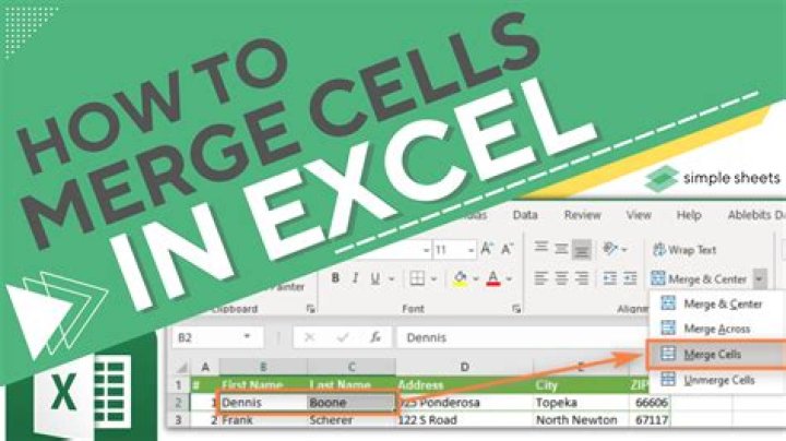
...and Excel will now properly ignore both header rows when auto-selecting the sort area:

Exceptions:

This obviously won't work if your first column requires both lines for headers, unless you're willing to live with one merged cell with two separate lines of text. While this will look fine, it's isn't semantically correct and could lead to problems in extreme edge cases if one assumes they are separate lines.

This also won't work if A1 is merged horizontally with B1, etc. There is no way around this problem unless you add a dummy column as the first column. If you can't do that, you will have to manually select all the data prior to sorting.

Note: all phone numbers were randomly generated with the formula below. Any similarity to an existing and valid number is purely coincidence.

=REPLACE(REPLACE(RANDBETWEEN(1000000000,9999999999),4,0,"-"),8,0,"-")

Excel 2007 can smartly detect if you have multi-row headers. I made a simple experiment just now before writing this.

Before making your first sort, position the cursor right below the header. That's it! Sorting is fine, filtering is fine. Excel ignored the 1st row of my headers. It just processes the 2nd row as the real header.

Highlight the cells that need to be sorted (all except the headers) and then select filter.

I am using Excel 2010. To retain the heading rows (e.g. the first 4 rows), highlight row 5 and then turn on the filters. Rows 1 - 4 are excluded from the filter.

I had the same issue, so everyone's contribution led me to the way the works for me (so far).

1. ADD a blank row below your Multi-row(s) Header (if your header is 5 rows of info and/or odd cell sizes, then your NEW blank row will be Row6).

2. Click on Row6 (to the far left/ actually click the "6" (Excel Row #) to select the entire row / to infinity). BE sure NOT to click any other CELL, until you have completed #3 and #4 below, or you will 'Deselect' the row. You want to keep it 'Selected'.

3. Go to the VIEW tab> Freeze Panes >Unfreeze (do this first to clear it) >Freeze. This will freeze your 5 row header & also the blank row (row6).

4. Hold Down "ALT", then press the following keys: D, F, F (this is the shortcut to turnON & turnOff/clear all filters on the sheet.

5. From this point forward, whenever you return to use this sheet & you need those Filters on (if you previously turned them off for any reason), then >Select your Blank Row (as explained in #2); >TurnON all your filters (as explained in #4).

Sorry to be so wordy, but after you do it a few times, will likely love it (if you use Filters a lot).

Step 1 Highlight the bottom header row. and then You can select just the cells in a row, or select the entire row.

Step 2 next click on "Sort & Filter" on the Home tab, then you can select "Filter." Excel adds filter arrows to all the column names.

Step 3 then click an arrow and later select a sorting option to sort the entire table by that column.

Step 4 finally click on "Sort & Filter" and select "Filter" again if you want to get rid of the arrows, but keep the sorting area defined by the filter. now you can sort normally, Excel ignores the extra header rows

Another way to accomplish in some cases is to enter a value in the second column that will cause the filter to include it, then make the text of that cell match the background colour of the cell. Not that pretty since the header (row 1) will not be horizontally centred in the cell but it will work...

I had the same problem and found a solution that works for me. For every row in the header that you don't want to see, you make te letters white (or the backgroundcolor). When you sort you don't see all the same headers in the rows. To bad when you want to change something, but in that case you can also make them light grey.