I have lots of data that looks like this. It has two columns:
| Name | |
|---|---|
| bob | |
| bob | |
| bob | |
| sally | |
| sally |
But I need it to look like this. One name per row, with the emails added as extra columns as required. There is an unknown number of emails for each name:
| Name | Email 1 | Email 2 | Email 3 |
|---|---|---|---|
| bob | |||
| sally |
I have to do this for a huge spreadsheet with thousands of rows. So I cannot manually convert each of them using something like transpose. I need a bulk/batch/automated solution.
I know that VBA is a thing that exists, but I don't know how to code it. If that is the solution can you please give me some direction of what the code should look like?
Non-VBA solutions are also very welcome.
4 Answers
Using Miller and starting from this CSV:
Name,Email bob, bob, bob, sally, sally, you can run:
mlr --csv nest --ivar ";" -f Email then nest --explode --values --across-fields -f Email then unsparsify input.csv >output.csv to obtain:
| Name | Email_1 | Email_2 | Email_3 |
|---|---|---|---|
| bob | |||
| sally | - |
Starting with your example Column A: Name , Column B: Email
- Enter this array formula:
=INDEX($A$2:$A$6, MATCH(0, COUNTIF($D$1:$D1, $A$2:$A$16), 0))into a blank cell, D2, for example, and press Shift + Ctrl + Enter keys together to get the correct result, see screenshot:
- Drag the cell down to fill in all values in column D. It will result like in the screenshot above.
- In cell E2 where you want your email insert this formula
=IFERROR(INDEX($B$2:$B$16, MATCH(0,COUNTIF($D2:D2,$B$2:$B$16)+IF($A$2:$A$16<>$D2,1,0),0)),"") - Drag the cell right 5-10 cells (or how much you consider is enough) to fill in and then drag the row down to fill in emails for each person.
Result:
1
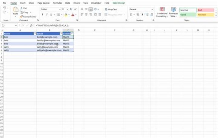
Add an auxiliary column with formula:
="Mail "&COUNTIF($A$2:A2,A2)
Open Power Query Editor - Select Column1- go to Transform- Pivot Column- select Email and under Advanced option select Don't Aggregate:
If you have new Excel version, you can use these formulas.
Then you can do it this way: The blue table is named Table1.
Used formulas:
- E3:
=UNIQUE(Table1[Name]) - F2:N2:
="Mail"&COLUMN()-COLUMN($E$2) - F3 (stretched down):
=INDEX(Table1[Mail];FILTER(TRANSPOSE(SORT(UNIQUE((ROW(Table1[Name])-ROW(Table1[[#Headers];[Name]]))*($E3=Table1[Name]))));TRANSPOSE(SORT(UNIQUE((ROW(Table1[Name])-ROW(Table1[[#Headers];[Name]]))*($E3=Table1[Name]))))>0;""))
Table is filled by SPILL function of the new Excel versions.
In case you are using older Excel version, most of the functionality could be emulated using array functions. But it becomes much more chaotic...
1