How do I ignore Empty Cells in the legend of a Chart or Graph

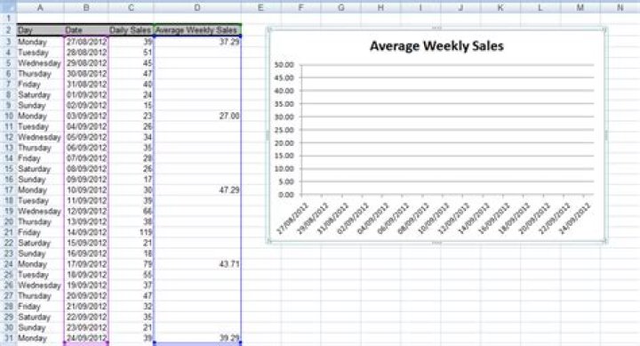
I am having trouble with a combination graph in excel specifically with the x axis. I have two columns both go to 1000 but currently only have 13 entries the rest will fill in over time.

I have a formula written to generate #N/A so there are no data points beyond the 13 that I currently have but the x axis still shows 1 to 1000 so the graph is unreadable.

How do I get the x axis labels to stop where the data stops rather than continuing out to 1,000?

Chart Example:

2 Answers

one approach to make it dynamic is to use named formula/range/cell. Instead of graphing A3:A1000 as your Series 1 Y values, you could assign A3:A1000 to the named range Series_1_Y. Edit your data for the graph and then edit the series and use the named range instead.

You can define names here:

That would be the basic concept of named range, but you need it to be more advanced and to be dynamic. There are a few way to achieve this. The basic thing you are going to need to do is determine the number of entries to include. Or in other words the number of rows. You can do this with the COUNT, COUNTIF, COUNTA and the like. You can then combine those results for use in something like OFFSET or INDEX.

In terms of using OFFSET or INDEX, offset is a volatile function, which means it recalculates everytime ANYTHING on the spreadsheet changes. INDEX on the other hand will only recalculate when when something that affects it changes. So depending on how frequently the formula gets used or the size of the calculation, INDEX won't bog your system down as much.

Since you do not have example data, I will work with the following layout:

You can count you entries in a variety of ways. two options are as follows:

=COUNT(A:A) or =COUNTIF(A3:A8,"<>#N/A") 'note the above only works for string version of NA 'and adjust characters to match your spelling 

The formula you will want to use in your "Define Name" formula will be something to the effect of:

=$A$3:INDEX($A$3:$A$8,COUNT($A:$A) or =OFFSET($A$3,0,0,COUNT($A:$A),1) 

Repeat the process for your second series changing the reference column

when working with your graph data you will need to have saved your spreadsheet first as your workbook name needs to be a part of the series name. I saved my work book as Dtest.xlsx and you can see the "Define Name" being used as the series below:

Note that if your workbook contains a space in the name surround the name in single quote/apostrophe as follows:

'Dtest Two.xlsx' 

Caveat: you cannot have any other numbers in the column and your numbers will need to be continuous from their starting point.

Perhaps the easiest way is to hide the columns (select the #N/A columns -> Right click -> Hide), they will not show on the graph.