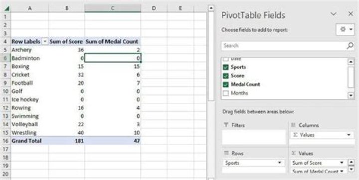
I've got two tables and two pivot tables for each of them respectively. In the first table, the duration of each task is calculated on a column called "duration", but in the second one, there is no such column and duration of each task is a calculated field in the pivot table. As you can see, in the first pivot table, tasks with zero time are not shown. But in the second pivot table, where durations are calculated fields, zero time tasks are shown as "0:00". How can I hide zero times like in the first table?
3 Answers
Right click on your PivotTable and select Pivot-Table Options, then use the For empty cells, show option - like here:
Ok, in case there is a Number like 0 or 00:00 in your Data and you don't want to display this too, you can solve it with a custom number format - like # or hh:mm:ss;hh:mm:ss;"";.
In excel's help you find this: <POSITIVE>;<NEGATIVE>;<NULL>;<TEXT> as the basic form for user-formats - so, this format here [h]:mm;[h]:mm;"";@ hides 00:00.
You can create a Calculated field in the formula box type : =IF(Value=0, "NA",Value) Now when there is a zero value it will force an error
Right click on your PivotTable and select Pivot-Table Options, then check the For error values, show option is ticked and blank
The added benefit of this method is the 0 value is not included in any totals or averages and the points will not print on any of the pivot charts
You can use conditional formatting for whole sheet or pivot area. Set new rule. "Format only cells that contain" and set "equal to 0" and set text color to white. Actualy it hides 0 but works.