Excel: How to do a count the number of cells that contain "X" AND have the cell above contain "Y"

I am an average user of Excel and this is a problem that I have encountered before and eventually found a different way to do it, but in this case I think it is my only option.

Here is a sample image of my sheet:

I want to count the number of times that a cell in the range contains "1a" AND the cell above the cell with 1a contains "Math". Obviously this example is trivial, but I figured the logic for solving this would be the same as if it were a larger worksheet with my data fully populating it.

In this example, the answer should be twice. How would I go about constructing a formula to make this type of conditional count?

6 Answers

You can use COUNTIFS formula. It allows you to specify multiple criteria. Using the example by pat2015, if the data is in range A3:J8, the formula should be

=COUNTIFS(A3:J7;"Math";A4:J8;"1a") 

(note the offset by one row between criteria)

I am proposing a solution that requires one Helper Column. Assuming your data is arranged in Cells A3:J8, use Column K as Helper and put the following Array Formula therein

{=SUM(IF($A4:$J4="1a",IF($A3:$J3="Math",1,0)))} 

Put the formula without Braces and then from within the Formula Bar press CTRL+SHIFT+ENTER to make it array formula. This gives count of '1a' with word 'Math' above that. Start in K4 say and drag it down. For alternate rows it will return 0 but that should not matter. Now just SUM the Helper Column. You can use simple SUM function for that. There might be smarter ways to achieve this without Helper column or one can even use VBA Macros.

If you reformat the data to have Math and 1a in the same cell:

=G5&" "&G6 

then you can use countif:

=COUNTIF($F$15:$K$18,N15) 

You can use:

=SUMPRODUCT(--(F3:K12&F2:K11="1a"&"Math"))

You have to use the initial Array (F3:K12) in the first reference and after & Your reference less one row (add one row up and less one row down) (F2:K11)
In that case (F3:K12&F2:K11="1a"&"Math") will return True if the rows in F3:K12 ="1a" and F2:K11="Math"
The -- in front of the condition will return 1 if it is True
Sumproduct will Sum (1,1,0...) Which is the count

=COUNTIFS(F3:K11, "Math", F4:K12, "1a") 

which has already been presented by fitch496, is a good start.  (Note: some locales use ; to separate function parameters; others use ,.)  It has one possible problem: it will count pairs of cells where “Math” is in an even-numbered row, and “1a” is below it in an odd-numbered row.  (While the question doesn’t speak to this issue, the illustration suggests that such pairs should not be counted.)

To resolve this issue, I started by translating the above formula into one that produces the same result, but using SUMPRODUCT:

=SUMPRODUCT(--(F3:K11="Math"), --(F4:K12="1a")) 

Here we use the standard tricks of preceding a Boolean expression by -- to turn TRUE into 1 and FALSE into 0, and using SUMPRODUCT’s implicit multiplication as a logical AND.  Then I extended that to

=SUMPRODUCT(--(F3:K11="Math"), --(F4:K12="1a"), --(MOD(ROW(F3:K11),2)=1)) 

to test that “Math” appeared in an odd-numbered row (MOD(ROW(…),2)=1).  This failed, because Excel seems to treat ROW(F3:K11) as the same as ROW(3:11), producing a linear array of 9 values rather than a rectangular array of 54 values.  (IMNSHO, this is a bug in Excel.)  I discovered that I could fix that by forcing it to take the columns into account, and then ignoring them:

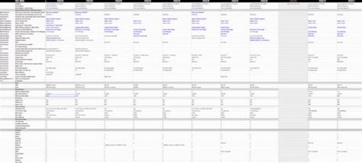
=SUMPRODUCT(--(F3:K11="Math"), --(F4:K12="1a"), --(MOD(ROW(F3:K11)+0*COLUMN(F3:K11),2)=1)) 

which evaluates the column number of each cell (COLUMN(…)) and then multiplies it by 0.  This works.  The illustration below is the same as the OP’s data in the question, but with the addition of “Math” and “1a” in cells J8 and J9.  fitch496’s COUNTIFS formula (which I include at the top of my answer) and my simple SUMPRODUCT formula both count this misaligned “Math 1a” and yield a total of 3; my final SUMPRODUCT formula ignores the misaligned “Math 1a” and yields a total of 2.

      
        ^{(See the source of this post for a copy-and-paste friendly copy of the above.)}

My formula can be streamlined a little:

• --(MOD(row number,2)=1) takes the row number modulo 2 and tests whether it’s equal to 1.  If it is, the comparison test yields a TRUE, which gets converted to 1 by --.  It it’s not 1, it must be 0; the comparison to 1 yields a FALSE, which gets converted to 0 by --.  We can dispense with the logic operations (testing for quality and then applying -- to the Boolean result) and just use MOD(row number,2).
• --(Boolean) is simply -(-(Boolean)).  The innermost - converts TRUE to 1 and FALSE to 0, but then it turns 1 into −1.  Then the outer - converts −1 back into 1.  Since we’re taking the product of two -- factors, the outer -s cancel each other out, so we can omit them.

So the final, streamlined formula is

=SUMPRODUCT(-(F3:K11="Math"), -(F4:K12="1a"), MOD(ROW(F3:K11)+0*COLUMN(F3:K11),2)) 

If you want to get total value that how many times both Math & 1a is written by single formula, it should be,

=COUNTIF (B86;E91, "Math") + Countif(B86:E91, "1a")

If want to count separately then same Countif,, formula twice.