I want to calculate the total amount of monthly fees based on the requirement price schedule below.
Price Schedule* – Monthly Fees per End User
1-100 end users: $29 each 101 - 250 end users: $27 each 251 - 500 end users: $25 each 501 - 750 end users: $23 each 750 - 1000 end users: $21 each 1001 - 1500 end users: $19 each 1501 - 2000 end users: $15 each 2001 - 2500 end users: $11 each 2501 - 5000 end users: $9 each 5001+ end users: $7 each *The prices apply to each customer in their respective tier. For clarity, the fee for the first 100 end users remains at $29 regardless of the total number of end users. The fee for the 101st to 250th end user is $27, and so on.
The input would be the number of end-users and the output would be the total monthly fees
An example would be 150 end users and the output would be:
(100*29) + (49*27) = 4,223 It is easy enough to manually calculate but really need a formula that is smart enough to calculate given just the number of end users
22 Answers
What I ended up doing was this formula. Not sure if this is the best way but seems to work
=(MIN(B1,100)*29)+ MAX(0,(MIN(250-100,(B1-100))*27))+ MAX(0,(MIN(500-250,(B1-250))*25))+ MAX(0,(MIN(750-500,(B1-500))*23))+ MAX(0,(MIN(1000-750,(B1-750))*21))+ MAX(0,(MIN(1500-1000,(B1-1000))*19))+ MAX(0,(MIN(2000-1500,(B1-1500))*15))+ MAX(0,(MIN(2500-2000,(B1-2000))*11))+ MAX(0,(MIN(5000-2500,(B1-2500))*9))+ MAX(0,(B1-5000)*7) This sort of issue is usually best served by a lookup table and the VLOOKUP function.
It allows for easier maintenance if things might change in the future.
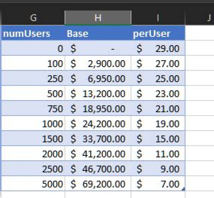
For example, set up your monthlyTable like this:
The first and third columns are entered manually. The Base column is computed with the formula:
H2: 0 H3: =(G3-G2)*I2+H2 Then you can use the formula:
B2: =VLOOKUP(A2,monthlyFees,2)+(A2-VLOOKUP(A2,monthlyFees,1))*VLOOKUP(A2,monthlyFees,3)